Context⌗

Picture this: there is a 3rd year undergraduate student trying to simulate a cloth. He have an elementary understanding of physics, differential equations, linear algebra, vector calculus and programming. He have a very crude experience of all this. He is a basic person. But this basic person wants to simulate clothes. What does he need to do. Well don’t wory because that basic person is me. And following is my struggle to simulate a cloth.

How do you simulate a cloth?⌗

How would you even start this? I thought of a straightforward way to do this. We’ll have many point masses and springs attached to them.

Here is an image of what it looks like:

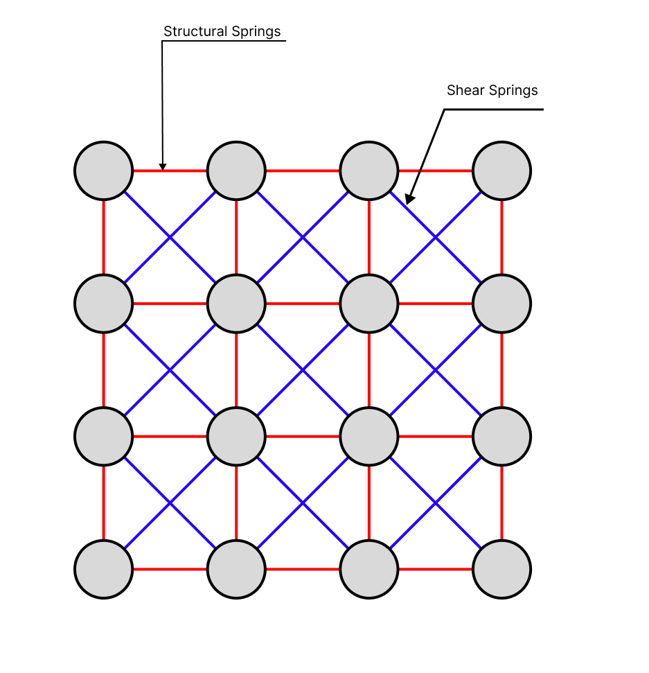
We have two types of springs here; the red ones are the structural springs, and the blue ones are the shear springs. The structural springs are attached to the adjacent points, and the shear springs are connected to the diagonal points. This is a simple model and should be very easy to implement. It was so easy, in fact, that I implemented a 2D version of this in an evening in processing. Here is how it looks:

That’s the extent of my ideas, but, surely people smarter than me would have done something better right? Yes, yes they have.

Let’s start with the basic stuff. This mass-spring system is actually a very good approximation of a cloth. People add a few more things to give it a bit more realism, and it being so computationally efficient is a huge plus.

One common trick is just to add a few more springs. These springs are called Bending Springs. These springs are attached to the second closest neighbours of a point. The real reason for doing this is actually because cloth does actually have bending stiffness, but who cares about that. I just follow the rule “The more the springs the better”.

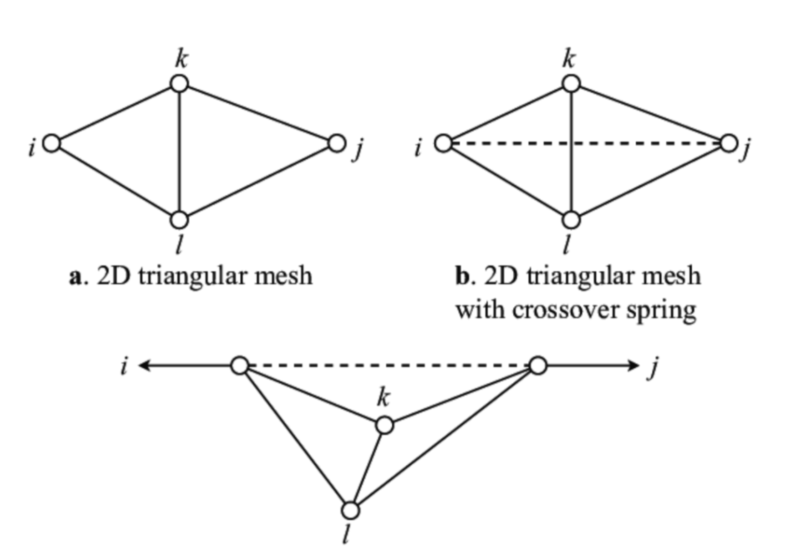
It’s also common to use triangular meshes. This is likely due to the fact triangles are better (and cooler!) than squares.

Now, because we have triangles, we don’t need shear springs. We can use the structural springs.

This is how a mesh like this would look like:

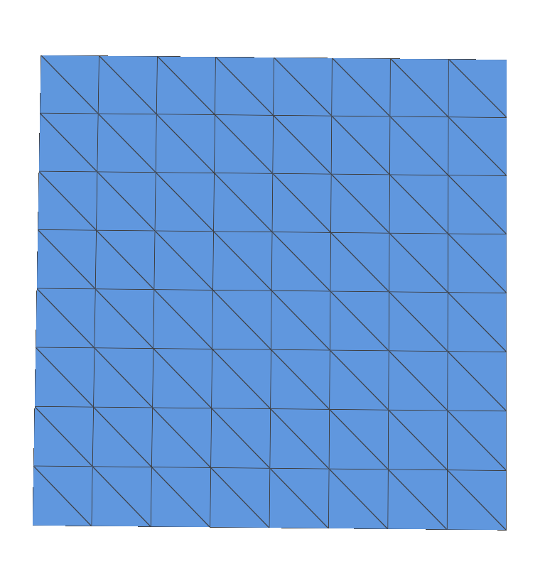
Above, you can see a simple cloth model with 25-point masses. Adjacent point masses have springs attached to them, these are the structural springs. The springs attached to the second closest neighbours are the bending springs.

To calculate the force on a point mass you just need to use hooke’s law.

\( \vec{F_P} = - C * \vec{v_P} - \sum_{Q \in R}{K_{PQ} * (|\vec{PQ}| - PQ_0) * \hat{PQ}} \)

\(\vec{F_P} := \) Internal Force at point \(P\).

\(R := \) Set of edges and second closest neighbours of \(P\).

\(K_{PQ} = K_{QP} := \) Spring constant along the edge \(P\).

\(\vec{PQ} := \) Vector connecting point \(Q\) with \(P\) \( = \vec{r_Q} - \vec{r_P} \).

\(\vec{r_P} := \) Vector to point \(P\).

\(PQ_0 := \) Initial length of the edge joining point \(P\) and \(Q\).

\(\hat{PQ} := \) Unit vector connecting point \(P\) and \(Q\).

\(\vec{v_P} := \) Velocity of point \(P\).

\(C := \) Damping Constant.

Simple stuff really. This is all just highschool maths.

So how do you solve this? Analytically, this would be a nightmare. It is a set of 2nd-order differential equations, I can’t even solve one such second order let alone a set of these. And apparently it actually is a really hard problem to solve analytically. Hence, we try to solve this numerically.

Numerically solving you need different time integration techniques, basically you throw away maths and become an engineer. It all starts with approximating derivatives \(\frac{dy}{dx} = \frac{\Delta y}{\Delta x}\). If you are a mathematician and are buthurt well I guess you can satisfy yourself with thinking this is just a first-order Taylor series approximation… but I am not a mathematician so I don’t care.

One such scheme is called Explicit Euler.

Explict Euler⌗

Simply put, we are going to use the current velocity and position of the point to calculate the next position and velocity of the point. This is done by using the following equations: \[ \vec{v_{P, t+1}} = \vec{v_{P, t}} + \frac{\vec{F_{P, t}}}{m} * \Delta t \] \[ \vec{r_{P, t+1}} = \vec{r_{P,t}} + \vec{v_{P, t}}\]

and obviously:

\( \vec{F_{P, t}} = - C * \vec{v_{P,t}} - \sum_{Q \in R}{K_{PQ} * (|\vec{PQ_{t}}| - PQ_0) * \hat{PQ_{t}}} \)

This is really cool and elegant the only problem is that it doesn’t work. It doesn’t work because it is not stable. This means that the system will just explode(if given no damping). This is because the system is doesn’t conserve energy.

You need to keep the time step really small for it to work. So we need to use a better method.

Implicit Euler⌗

Implicit Euler is a better method. It is stable as in it decreases energy over time, hence it is impossible to explode. But it is a bit more complicated. The only equation which changes is the velocity equation. \[ \vec{v_{P, t+1}} = \vec{v_{P, t}} + \frac{\vec{F_{P, t+1}}}{m} * \Delta t \]

This uses the next positions to calculate the next velocities. This is a bit more complicated to solve. Since we are using the next positions to calculate the next velocities we need to solve a system of equations. So how do you even calculate the next positions? This is like the chicken and egg problem but with differential equations. How do you get the next positions if you don’t have the next velocities? How do you get the next velocities if you don’t have the next positions?

Well the answer is obvious really: \[ \vec{F_{P,t+1}} = \vec{F_{P, t}} + \frac{\partial{\vec{F_P}}}{\partial{\vec{r_P}}} * \Delta \vec{r} + \frac{\partial{\vec{F_P}}}{\partial{\vec{v_Q}}} * \Delta \vec{v}\]

You just use the first-order Taylor series expansion of a multivariable vector function… duh.

So I guess I need to do this \(\forall P\) and we’re done? Well that’s a bit anti-climatic. I mean I was expecting something more complicated. But I guess this is it.

A Nightmare peaking from the horizon⌗

So well turns out this is slightly more involved. After watching tons of lectures on vector calculus and understanding what it even means to differentiate a vector with another vector I was able to start to understand what was going on.

Basically when you differentiate a vector with another vector you get a matrix, this is also called jacobian and I will be using these two interchangeably from now on. This matrix, when you differentiate force with direction, is usually supposed to be material property.

In highschool you must have read about hooke’s law:

\( e = \frac{E\epsilon^2}{2} \)

Where \(e = \) strain energy, \(E = \) Young’s Modulus and \(\epsilon = \) strain.

you differentiate this and get:

\(\sigma = E\epsilon\)

Where \(\sigma = \) stress.

one more time and you get: \(\frac{\partial{\sigma}}{\partial{\epsilon}} = E\)

As you can see this is a material property. Similary in this case we have a material property. This matrix is of 3x3 for each point.

So all you have to do is get this matrix. Thankfully people much more intelligent then me have calculated this. Infact it is assumed that you’ll provide this matrix whenever you publish a new material model. Yes there are many more material models and they have different approaches. But all just essentially either change the forces on the points, or use FEM.

What you can even do is write all these equations in one big matrix and then use sparse matrix solving techniques like conjugate gradient and just like that you have a cloth simulator. Easy right?

Anyways with this I was able to get some cool results. Here is an example simulation:

The end of the simulation:

But this doesn’t feel enough I want more realism. So I looked across various ways to make more realistic cloth and find one interesting model.

This is the Bridson Bending Model. Which was published in this paper.

Okay so it starts with focusing on only 2 triangles and is somehow trying to implement repulsions based on the angle between these “triangular flaps”. This is a pictorial representation of what I am talking about:

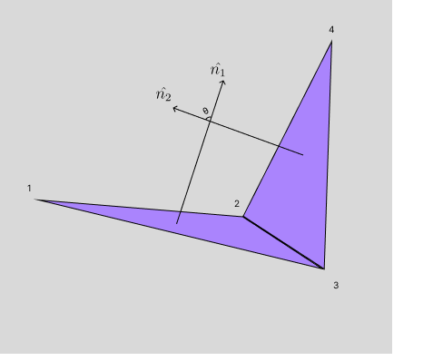
The angle between the two triangles is \(\theta\).

\[ \vec{F_i} = K\frac{|{\vec E}|^2}{|{\vec N_1}| + |{\vec N_2}|} (sin(\theta/2) - sin(\theta_0 / 2)) {\vec u_i}\]

\(F_i := \) The force on the ith point mass (\(i \in \{ 1,2,3,4 \}\)).

\[{\vec E} := {\vec x_4} - {\vec x_3}\] \[{\vec N_1} := ({\vec x_1} - {\vec x_3}) \times ({\vec x_1} - {\vec x_4})\] \[{\vec N_2} := ({\vec x_2} - {\vec x_4}) \times ({\vec x_2} - {\vec x_3})\] \[sin(\theta/2) = \pm \sqrt{\frac{(1 - \hat{n_1} \cdot \hat{n_2})}{2}}\]

\( {\vec x_i} := \) Position of the ith point mass. \( {\vec u_i} := \) Instantaneous direction of the ith point mass.

Great… So is their a closed form for \({\vec u_i’s}\)

Ofcourse, here they are: \({\vec u_1}\) and \({\vec u_2}\) are in the direction of \({\vec N_1}\) and \({\vec N_2}\) respectively. That makes sense.

\[{\vec u_1 } = |{\vec E}| \frac{\vec N_1}{|{\vec N_1}|^2} \] \[{\vec u_2 } = |{\vec E}| \frac{\vec N_2}{|{\vec N_2}|^2} \]

And for \({\vec u_3}\) and \({\vec u_4}\) we have:

\({\vec u_3 } = \frac{({\vec x_1 - x_4}) \cdot {\vec E}}{|{\vec E}|} \frac{\vec N_1}{|{\vec N_1}^2|} + \frac{({\vec x_2 - x_4}) \cdot {\vec E}}{|{\vec E}|} \frac{\vec N_2}{|{\vec N_2}|^2}\)

\({\vec u_4 } = -\frac{({\vec x_1 - x_3}) \cdot {\vec E}}{|{\vec E}|} \frac{\vec N_1}{|{\vec N_1}^2|} - \frac{({\vec x_2 - x_3}) \cdot {\vec E}}{|{\vec E}|} \frac{\vec N_2}{|{\vec N_2}|^2}\)

….

I can’t even understand this, how do you even differentiate that. I am just happy I am not the one who’s going to be doing that. Let’s just quickly implement this for our explicit euler version with damping(the one without differentiations) and see what happens.

Here is the result:

Okay that looks better and more cloth like. Let’s see what happens when we add bending to the implicit euler. Let’s quickly look for the jacobians and… wait…

THERE ARE NO JACOBIANS

The following is my stream of consciousness and thoughts while I was trying to figure out how to do this. For more concrete thoughts checkout my short note on jacobian calculation of this problem:

Calm before the storm⌗

So there are no force derivatives for this… Hence we’ll have to do this on our own. This task is very daunting, and I don’t even know where to start.

Well let’s just have a go at it. How hard can it be?

First let’s divide and conquer. I guess it works pretty well, the british did it and they conquered half the world. I can atleast find these derivatives…

Here is my strategy, I’ll find Derivative of this equation: \[{\vec F_i} = K A_0 {\vec u_i}\] With \(A_0 := \frac{|{\vec E}|^2}{|{\vec N_1}| + |{\vec N_2}|} (sin(\theta/2) - sin(\theta_0 / 2)) \)

For this I only need derivative of \(A_0\) and \({\vec u_i}\).

Let’s start with \(A_0\).

Even this seems daunting so let’s define \(A_1\). \[A_1 := \frac{|{\vec E}|^2}{|{\vec N_1}| + |{\vec N_2}|}\]

Finally something which seems easy enough to differentiate.

To do this we’ll require the derivatives of \(|{\vec E}|\), \(|{\vec N_1}|\) and \(|{\vec N_2}|\) wrt to the position of the point masses.

Let’s start with \({\vec E}\).

\[{\vec E} := {\vec x_4} - {\vec x_3}\]

okay… wait how would you do this? so let’s see if highschool’s vector addition taught me anything it was \( |{\vec E}| = \sqrt{|{\vec x_4}|^2 + |{\vec x_3}|^2 - 2 {\vec x_4} \cdot {\vec x_3}} \).

Clearly \(\frac{\partial |{\vec E}|}{\partial {\vec x_1}} = \frac{\partial |{\vec E}|}{\partial {\vec x_2}} = 0\)

Instead of finding the derivative of \(|{\vec E}|\) let’s find the derivative of \(|{\vec E}|^2\).

After all \(\frac{\partial |{\vec E}|}{\partial {\vec x_j}} = \frac{1}{2|{\vec E}|} \frac{\partial |{\vec E}|^2}{\partial {\vec x_j}}\)

I’ll spare you the maths but here is the result: \[\frac{\partial |{\vec E}|}{\partial {\vec x_3}} = \frac{{\vec x_3}^T - {\vec x_4}^T}{|{\vec E}|}\] \[\frac{\partial |{\vec E}|}{\partial {\vec x_4}} = \frac{{\vec x_4}^T - {\vec x_3}^T}{|{\vec E}|}\]

Okay now with \(N_1\) and \(N_2\). And I’m stuck… I don’t even know how you’ll differentiate a cross product. I can use indical notation but that’s a whole lot of headache that I don’t really want to get into… I just want to animate a cloth. I scrolled through pages and pages of vector calculus and I couldn’t find anything other than this stack overflow… But what even is this notation. I have no idea what this skew() function is. After searching for more information on this I gave up, wrote this problem to few of my friends and just hoped for the best, then someone actually came through. Apparently this skew() function takes in a vector cross product and makes it into a matrix product. Which obviously can be differentiated by using the product rule.

So this is how this magic works: \({\vec a} \times {\vec b} = - {\vec b} \times {\vec a} = - skew({\vec b}){\vec a} \implies \frac{\partial( {\vec a} \times {\vec b} )}{\partial {\vec a}} = \frac{\partial( -skew({\vec b}){\vec a} )}{\partial {\vec a}} = -skew({\vec b})\). This identity holds \(\forall\) independent \(a, b\).

\[skew({\vec b}) := \begin{pmatrix} 0 & -b_3 & b_2 \\ b_3 & 0 & -b_1 \\ -b_2 & b_1 & 0 \end{pmatrix}\]

With this we can finally get the derivatives of \(|{\vec N_1}|\) and \(|{\vec N_2}|\), by using the fact: \[\frac{\partial |{\vec N_i}|}{\partial {\vec x_j}} = \frac{\partial |{\vec N_i}|}{\partial {\vec N_i}} \frac{\partial {\vec N_i}}{\partial {\vec x_j}} = {\hat{n_i}^T} \frac{\partial {\vec N_i}}{\partial {\vec x_j}} \]

and sparing the maths, now you can get all the \(\frac{\partial {\vec N_i}}{\partial {\vec x_j}}\).

Now all I need to work out is how this product situation is going to work… Well we can use this clever log trick:

\[ log(A_1) = 2log(|{\vec E}|) - log(|{\vec N_1}| + |{\vec N_2}|) \]

\[\implies \frac{1}{A_1}\frac{\partial A_1}{\partial {\vec x_i}} = \] \[\frac{2}{|{\vec E}|} \frac{\partial |{\vec E}|}{\partial {\vec x_i}} - \frac{1}{|{\vec N_1}| + |{\vec N_2}| }\frac{\partial (|{\vec N_1}| + |{\vec N_2}| )}{\partial {\vec x_i}} \]

This makes it so much more easier to deal with.

Now I can move into the next part of the equation, \({\vec u_i}\).

Surely I can use something similar right? I mean all I need is a log equivalent for a vector… well I can use component wise log.

This is how it works: since all \(u_i\) is of the form scalar * vector or sums of these, we can easily use this to calculate derivatives.

Let, \[ {\boldsymbol {\phi}} = {\vec a} \prod_{k = 1}^{n} C_k\]

Taking log and then differentiating wrt to ({\vec x_j}) we get the following equation equating two row vectors:

\[ \frac{1}{\phi_i} \frac{\partial {\phi_i}}{\partial {\vec x_j}} = \sum_{k=1}^n\frac{1}{C_k} \frac{\partial C_k}{\partial {\vec x_j}}+ \frac{1}{a_i} \frac{\partial {a_i}}{\partial {\vec x_j}}\]

Doing this I can get all the derivatives of \({\vec u_i}\). Infact, it’s even better we can also verify that at runtime if \({\vec u_i}\)’s derivative’s are correct or not. \(\sum_{i=0}^4{\frac{\partial {\vec u_i}}{\partial x_j}} = 0\). So that’s neat.

Now only thing left is to get the derivative of \(sin(\theta/2)\).

Let’s try with getting derivative of \(\hat{n_1}\) and \(\hat{n_2}\) wrt to \({\vec x_j}\).

After tireless calculations… I did manage to calculate this. It’s ugly and bad and just plain looks shady, but well it is what it is and finally I can finally get the force derivative…. wrt. positions atleast.

Velocity would be similar but that’s future me’s problem. For now let’s ignore daming and see our beautiful cloth simulate and…..

It explodes

The Nightmare⌗

Working in tech things are bound to go wrong. Everything that can go wrong does eventually find a way to come back and haunt you when you expect it the least.

First question: Why did it explode? Second Question: How do I fix it? How do you even debug it?

Well let’s start with the first question. Why did it explode? There can only be two things, first one is easy. I did a typo, maybe some multiplication was suppposed to be inside a parenthesis and it wasn’t. Or maybe I forgot to add a negative sign somewhere. Or maybe I just forgot to add a term. These are easy to debug, you just go through the code and see if you can find any mistakes. But a scary 2nd option was in the view… what if the maths is wrong.

At this point for refrence I have spent over 3-4 weeks just trying to get these jacobians. Calculating these are no small task especially the \(sin(\theta / 2 )\) that took enormous hours and I was so happy when I finally got it. But what if it was wrong? What if I made a mistake somewhere and I just didn’t notice it. I mean I am not a mathematician,I am not even a physics major.

So how do you debug this?

When all hope was lost. Something struck. You can approximate the derivative numerically, and then check if it’s correct or not.

So I implemented it and lo and behold it was wrong. I was so happy that it was wrong. I checked for all the components and found many many of them were eitehr typos or mathematically wrong. After tirelessely fixing all these I was finally at the end. I had fixed everything. The difference between the numerical approximation and my analytic derivatives was meagre. I was so happy. I was finally done. I was finally going to see my cloth simulate and it EXPLODED…. It exploded? what? but… The jacobians are correct? how can it explode…

Sometimes while debugging you hit such a wall that you don;t even know how to proceed. What can even be wrong? I mean I have checked everything. I have checked the jacobians, I have checked the equations, I have checked the code. I have checked everything. What can even be wrong? I ran a debugger as a last hope seeing if I can find anything being wrong, nothing. Everything was working as expected.

That’s when it dawned me. What if all this time my forces were wrong… what if I made a mistake in the force calculation.

I checked the force calculation and lo and behold I had made huge errors looking back at that was almost astonishing how many silly mistakes I HAD MADE. I DON;T EVEN KNWO HOW THE jacobians were, correctly, approximating this.

Here are the most ridiculous mistakes I had made:

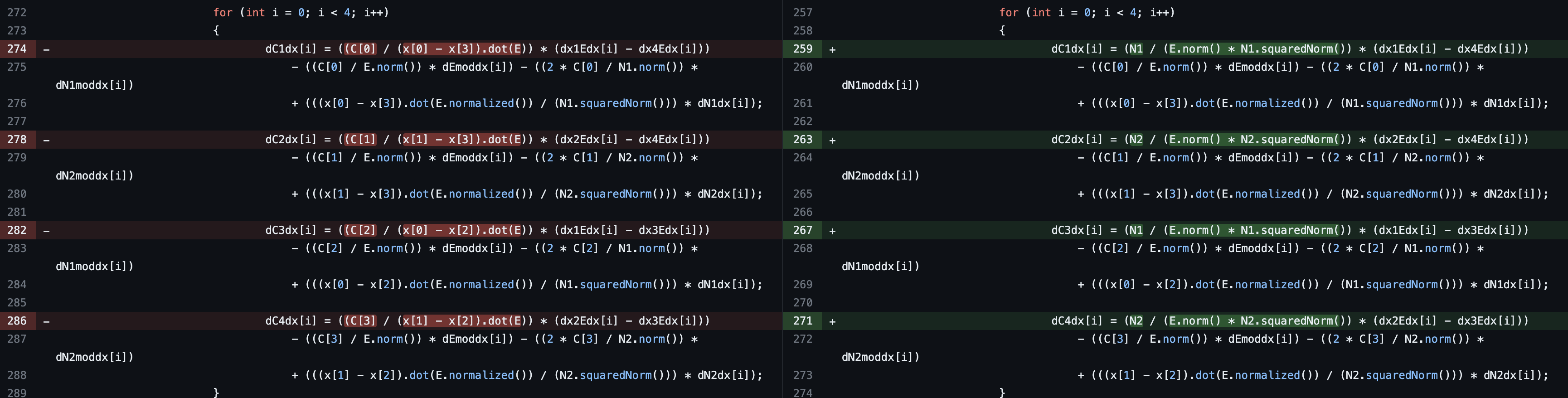
The list goes on but I was finally able to fix it. So finally, finally my cloth sim can work….

And it explodes again… This time it goes NAN. Hmm… this is weird…

All’s well that ends well⌗

That’s when it clicked. The reason why this \(sin(\theta / 2)\) looks so weird, we had a square root in it. It can possibly go negative. And it does, because of floating point errors. So I need to check if it’s really close to zero. I did it and it doesn’t explode so that’s cool. But the jacobians still do not approximate forces. Hmm… looking deeply into it I found out that the jacobians are still going NAN and the culprit… the same square root.

The only solution is hence that this form is very poor. That’s when I gave up and started implementing Damping… afterall it’s not exploding at small timestep right?

Implementing damping I notice a formula: \[\frac{d\theta}{dt} = {\vec u_1} \cdot {\vec v_1} + {\vec u_2} \cdot {\vec v_2} + {\vec u_3} \cdot {\vec v_3} + {\vec u_4} \cdot {\vec v_4}\]

This is equivalent to saying: \[\frac{\partial \theta}{\partial {\vec x_i}} = {\vec u_j}\] And this means that the answer was here right along: \[\frac{\partial sin(\theta / 2)}{\partial {\vec x_j}} = \frac{cos(\theta / 2)}{2} {\vec u_j} \]

And: \[cos(\theta / 2) = + \sqrt{\frac{1 + \hat{n_1} \cdot \hat{n_2}}{2}}\]

All this so elegant and compact. And the jacobian is simple enough that having floating point errors is easily fixable.

After all this… finally my implicit euler simulation works!

It works and it’s glorious.